Bivariate histograms

Histograms are a great way to get an overview of the information distribution of an image. This notebook shows how to create bivariate histogram with and without logarithmic scaling.

What you need to produce this histogram is

Two images (n and x) and

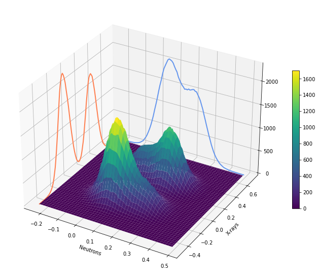
• the numpy functions histogram and histogram2d:

  H, xedges, nedges = np.histogram2d(x.ravel(), n.ravel(), bins=nBins)
  nH,nax = np.histogram(n.ravel(),bins=nedges)
  xH,xax = np.histogram(x.ravel(),bins=xedges)
  

• the matplotlib function plot_surface imported using from mpl_toolkits.mplot3d import Axes3D:

  X, Y = np.meshgrid(xedges[:-1], nedges[:-1])
  fig = plt.figure(figsize=(12,10))
  ax = fig.gca(projection = '3d')
  hScale = 0.05
  ax.plot(nedges[:-1], hScale*xH, zs=xedges.min(), zdir='x', lw = 2., color = 'coral')
  ax.plot(xedges[:-1], hScale*nH, zs=nedges.max(), zdir='y', lw = 2., color = 'cornflowerblue')
  cax=ax.plot_surface(X, Y, H, cmap='viridis')
  fig.colorbar(cax,shrink=0.5)
  ax.set_ylabel('X-rays');
  ax.set_xlabel('Neutrons');
  plt.show()